Quick start: ground state calculation for benzene#
Postopus (the POST-processing of Octopus data) is an environment that can help with the analysis of data that was computed using the Octopus TDDFT package.
In this notebook we give some quick examples how easy you can access data of Octopus using Postopus. The notebook assumes that you have Octopus installed and is in your (bash) path.
Running the simulation#
Octopus takes an input file describing the systems and the simulation parameters. The input file is called inp and is a text file with no extension.
(The !command IPython Magic lets us execute bash commands in the notebook.)
Create the directory in which we run octopus:
[1]:
!mkdir -p "examples/benzene"
[2]:
cd "examples/benzene"
/builds/lang-m/postopus/docs/notebooks/examples/benzene
Now create the inp file. This is achieved with the `%%writefile <https://ipython.readthedocs.io/en/stable/interactive/magics.html#cellmagic-writefile>`__ magic command:
[3]:
%%writefile inp
stdout = "gs_stdout.txt"
stderr = "gs_stderr.txt"
CalculationMode = gs
UnitsOutput = eV_Angstrom
Radius = 5*angstrom
Spacing = 0.15*angstrom
%Output
wfs
density
elf
potential
%
OutputFormat = cube
OutputDuringSCF = yes
OutputInterval = 5
XYZCoordinates = "benzene.xyz"
FromScratch = true
Writing inp
Similarly we define the geometry file (benzene.xyz):
[4]:
%%writefile benzene.xyz
12
Geometry of benzene (in Angstrom)
C 0.000 1.396 0.000
C 1.209 0.698 0.000
C 1.209 -0.698 0.000
C 0.000 -1.396 0.000
C -1.209 -0.698 0.000
C -1.209 0.698 0.000
H 0.000 2.479 0.000
H 2.147 1.240 0.000
H 2.147 -1.240 0.000
H 0.000 -2.479 0.000
H -2.147 -1.240 0.000
H -2.147 1.240 0.000
Writing benzene.xyz
Now we can invoke octopus:
[5]:
!octopus
[ 15/ 15] 100%|*************************************************| 00:00 ETA
Octopus stores the calculation results in the project directory. If you were to take a look at the benzene project folder, you would see something like:
├── benzene.xyz # Geometry of the molecules (input)
├── exec # Runtime information
│ ├── initial_coordinates.xyz
│ ├── messages
│ ├── oct-status-finished
│ └── parser.log # Full set of variables used for the run
├── inp # Our input file
├── out_gs.log # Log file
├── output_iter # Output for each iteration in scf/td calculation
│ ├── scf.0005
│ │ ├── density.cube
│ │ └── ...
│ └── scf.0010
│ ├── density.cube
│ └── ...
├── restart
│ └── gs # Ground state calculations
│ ├── 0000000001.obf # Checkpoint file to restart calculation in case of job abortion
│ ├── 0000000002.obf
│ ├── ...
│ └── wfns
└── static # Ground state observables
├── info # Result of ground state calculation (like energy eigenvalues and forces)
├── convergence
├── density.cube
├── ...
└── wf-st0015.z=0
These new files are the results of the simulation. We will now analyse the output files to examine the simulation results. The Postopus package helps in this part.
Postopus#
First, we have to import the Octopus run using Postopus:
[6]:
from postopus import Run
run = Run(".") # or equivalent run = Run()
System selection#
Now we have to select the system. To list available systems we print the run object. If the multisystem feature of Octopus is not used, Postopus uses the name “default”.
[7]:
run
[7]:
Run('/builds/lang-m/postopus/docs/notebooks/examples/benzene'):
Found systems:
'default'
Found calculation modes:
'scf'
Calculation modes#
We can take a look at the different types of calculations done in this system by running:
[8]:
run.default
[8]:
System(name='default', rootpath='/builds/lang-m/postopus/docs/notebooks/examples/benzene'):
Found calculation modes:
'scf'
This tells us that this project had only a self-consistent field simulation (scf).
Outputs#
Printing the calculation mode gives us a list of available outputs:
[9]:
run.default.scf
[9]:
CalculationModes('scf'):
Ground state calculation (finished after 18 steps)
Found 10 outputs:
convergence
density
elf_rs
forces
info
v0
vh
vks
vxc
wf
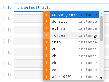
Autocompletion#
The tab completion feature available in Jupyter notebooks and IPython supports navigating the systems, calculation modes and outputs. Here is an example image of how the tab completion feature works:
Output files#
Postopus makes all the files of the Octopus simulation easily accesible. The data is provided mostly as pandas DataFrame or xarray DataArray/Dataset:
Table-like structured files#
We can take a look at the convergence of the systems energy after each scf iteration through:
[10]:
run.default.scf.convergence()
[10]:
| energy | energy_diff | abs_dens | rel_dens | abs_ev | rel_ev | |
|---|---|---|---|---|---|---|
| #iter | ||||||
| 1 | -1266.189500 | 1266.190000 | 6.576180 | 2.192060e-01 | 24.450600 | 0.046511 |
| 2 | -1186.519650 | 79.669800 | 0.727949 | 2.426500e-02 | 71.843200 | 0.158294 |
| 3 | -946.223309 | 240.296000 | 2.574540 | 8.581790e-02 | 134.692000 | 0.422011 |
| 4 | -1066.186400 | 119.963000 | 1.242070 | 4.140220e-02 | 72.969600 | 0.186083 |
| 5 | -1060.008750 | 6.177660 | 0.168404 | 5.613460e-03 | 10.448500 | 0.027374 |
| 6 | -1029.952950 | 30.055800 | 0.331029 | 1.103430e-02 | 15.929100 | 0.043551 |
| 7 | -1018.415290 | 11.537700 | 0.136615 | 4.553840e-03 | 4.685590 | 0.012977 |
| 8 | -1024.289710 | 5.874410 | 0.065752 | 2.191730e-03 | 3.171370 | 0.008707 |
| 9 | -1028.835710 | 4.546000 | 0.049664 | 1.655480e-03 | 2.256280 | 0.006156 |
| 10 | -1027.860460 | 0.975253 | 0.011123 | 3.707720e-04 | 0.720237 | 0.001969 |
| 11 | -1026.552430 | 1.308020 | 0.013103 | 4.367710e-04 | 0.722050 | 0.001978 |
| 12 | -1026.607480 | 0.055050 | 0.001182 | 3.941570e-05 | 0.080786 | 0.000221 |
| 13 | -1026.740610 | 0.133125 | 0.001377 | 4.589510e-05 | 0.078020 | 0.000214 |
| 14 | -1026.746600 | 0.005996 | 0.000277 | 9.239740e-06 | 0.003708 | 0.000010 |
| 15 | -1026.748140 | 0.001535 | 0.000091 | 3.029840e-06 | 0.001447 | 0.000004 |
| 16 | -1026.735580 | 0.012563 | 0.000136 | 4.537000e-06 | 0.007057 | 0.000019 |
| 17 | -1026.736370 | 0.000793 | 0.000026 | 8.554120e-07 | 0.000665 | 0.000002 |
| 18 | -1026.737440 | 0.001073 | 0.000024 | 8.062470e-07 | 0.000586 | 0.000002 |
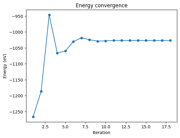
If we wanted to visualize the convergence of the energy, we can run the following:
[11]:
# Plot of energy at each interaction showing its convergence
fig = run.default.scf.convergence()["energy"].plot(
title="Energy convergence",
marker=".",
markersize=10,
)
fig.set(xlabel="Iteration", ylabel="Energy (eV)");
Fields#
We can simply load the data of the output accross all iterations (including the output in static/):
[12]:
density_data = run.default.scf.density("cube")
density_data
[12]:
<xarray.DataArray 'density' (step: 4, x: 95, y: 99, z: 67)> Size: 20MB
[2520540 values with dtype=float64]
Coordinates:
* step (step) int64 32B 5 10 15 18
* x (x) float64 760B -13.32 -13.04 -12.76 -12.47 ... 12.76 13.04 13.32
* y (y) float64 792B -13.89 -13.61 -13.32 -13.04 ... 13.32 13.61 13.89
* z (z) float64 536B -9.354 -9.071 -8.787 -8.504 ... 8.787 9.071 9.354
Attributes:
units: auThe data object is an xarray object containing not only the data values, but also the coordinates for which these values are defined:
[13]:
density_data.coords
[13]:
Coordinates:
* step (step) int64 32B 5 10 15 18
* x (x) float64 760B -13.32 -13.04 -12.76 -12.47 ... 12.76 13.04 13.32
* y (y) float64 792B -13.89 -13.61 -13.32 -13.04 ... 13.32 13.61 13.89
* z (z) float64 536B -9.354 -9.071 -8.787 -8.504 ... 8.787 9.071 9.354
For more information on the units take a look at the units tutorial.
Working with the data: Xarray#
First, let us access the data from the last iteration only:
[14]:
xa = density_data.isel(step=-1)
xa
[14]:
<xarray.DataArray 'density' (x: 95, y: 99, z: 67)> Size: 5MB
[630135 values with dtype=float64]
Coordinates:
step int64 8B 18
* x (x) float64 760B -13.32 -13.04 -12.76 -12.47 ... 12.76 13.04 13.32
* y (y) float64 792B -13.89 -13.61 -13.32 -13.04 ... 13.32 13.61 13.89
* z (z) float64 536B -9.354 -9.071 -8.787 -8.504 ... 8.787 9.071 9.354
Attributes:
units: auIn the first line of output of the previous cell, we can see an overview of the Xarray data inside the density field. The first line tells us the number of sampling points in each direction:
xarray.DataArray ‘density’ (x: 95, y: 99, z: 67)
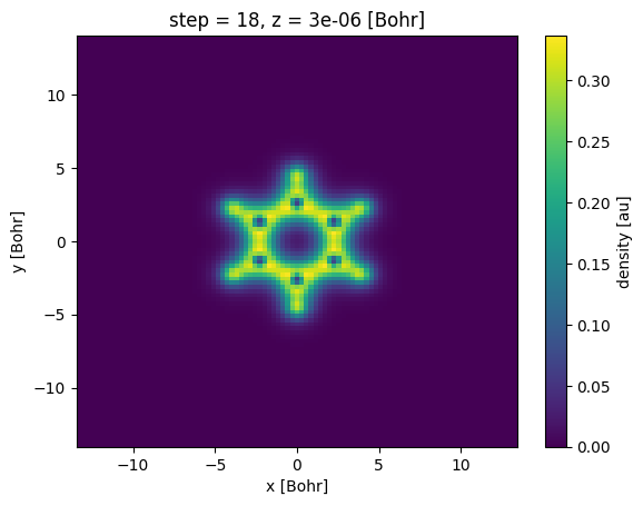
So there are 95 sampling points in the x-direction and similarly 67 for the z-direction. Suppose we want to have a view of density of benzene in the x-y plane (i.e. at \(z=0\)), we can do so by selecting the slice at z=0. One way to do this for this particular simulation is by asking Xarray for selecting the slice at the index \(i_z=67/2~\approx~33\):
[15]:
s0 = xa.isel(z=33) # Viewing the slice at 33rd index of z-axis
s0
[15]:
<xarray.DataArray 'density' (x: 95, y: 99)> Size: 75kB
[9405 values with dtype=float64]
Coordinates:
step int64 8B 18
* x (x) float64 760B -13.32 -13.04 -12.76 -12.47 ... 12.76 13.04 13.32
* y (y) float64 792B -13.89 -13.61 -13.32 -13.04 ... 13.32 13.61 13.89
z float64 8B 3e-06
Attributes:
units: auThis slice returns another Xarray object. Note here that the coordinate value for z is 3e-06, which is the value of z coordinate for the 33rd sampling point in the z-direction. We can now plot this slice using the plot() method of the Xarray object:
(The ; after s0.plot() is a trick used to prevent IPython from printing the result of s0.plot() which would show something like <matplotlib.collections.QuadMesh at 0x7f181bbf8a10> above the actual plot.)
[16]:
s0.plot();

Note that the plot has the x and the y axis inverted, one can change this by passing the x='x' argument to the plot() method.
[17]:
s0.plot(x="x");

Another way to slice the data is by using the sel() method of the Xarray object, where you can pass the coordinate value instead of the index.
For example, to get the same slice as above, we can use:
[18]:
s1 = xa.sel(z=0, method="nearest")
s1.plot(x="x");
Note that plots automatically display the value of the position of the slice in the z-direction as well as the step number. This is possible because Xarray maintains the metadata of the coordinates even after slicing.
One can have a side view of the molecule by slicing the data in the y-z plane (e.g. at \(x=0\)) in a similar fashion:
xa.sel(x=0, method='nearest')
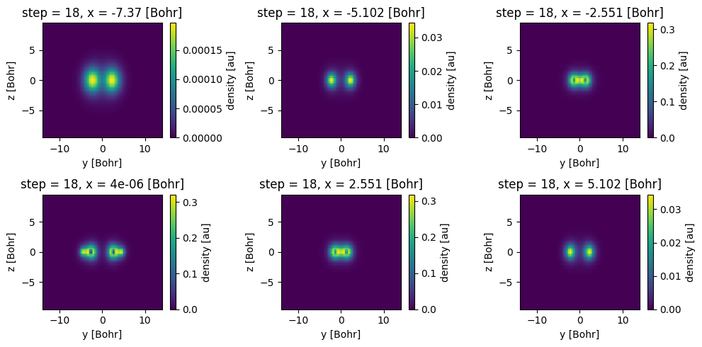
Using a for loop and some commands from the matplotlib plotting library, we can plot 6 different slices of the data in a 3x2 grid at different values of x.
[19]:
import numpy as np
import matplotlib.pyplot as plt
# create a subplot with 2 rows, 3 columns
fig, axs = plt.subplots(2, 3, figsize=(10, 5))
# x positions from -7.5 to 5 in 6 steps
x_positions = np.linspace(-7.5, 5, 6)
for ax, x in zip(axs.flat, x_positions):
# plot the slice nearest to x position
xa.sel(x=x, method="nearest").plot(ax=ax, x="y")
fig.tight_layout() # avoid overlap of labels
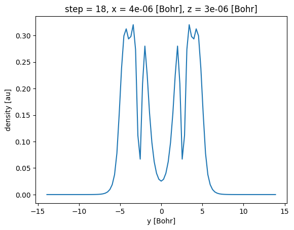
The sel method can also be used to select a multiple coordinates at once, for example to select the slice at \(x=0\) and \(z=0\) we can do:
xa.sel(x=0, z=0, method='nearest')
We can then plot the variation of density along the y axis. Because we have restricted two (x and z) of the three spatial dimensions, we obtain a ‘line plot’ of the density along the remaining coordinate dimension y.
[20]:
xa.sel(x=0, z=0, method="nearest").plot()
[20]:
[<matplotlib.lines.Line2D at 0x7fba20547f50>]
A more detailed exploration of plotting with Xarray is available in the postopus plotting tutorial.
Plotting with holoviews#
A plotting library that is built for interactive/multidimensional plots is holoviews. Converting xarray objects (the most common output type in postopus) to holoviews objects is simple, as we will see. Holoviews supports many backends for plotting. In this tutorial we will use bokeh (the default plotting backend for holoviews).
The holoviews approach to plotting may seem unconventional (and perhaps confusing) at first — it is, however, very powerful. In particular, holoviews allows the selective and/or interactive visualization of data that is defined in more dimensions that we can easily visualize. To be able to use that power, we need to provide some additional information to the plotting commands: for example which of the many dimensions we want to plot, and for which we would like to have an interactive slider to select it.
We provide a few examples that can be used as templates to cover typical use cases below.
First, let us import the holoviews library as well as the plotting backends we will use:
[21]:
import holoviews as hv
from holoviews import opts # For setting defaults
hv.extension("bokeh") # Allow for interactive plots


We then choose the color map we want to use for the plots. We use viridis.
[22]:
# Choose color scheme similar to matplotlib
opts.defaults(
opts.Image(cmap="viridis", width=400, height=400),
)
Now we can plot our density data including sliders to easily explore the data:
[23]:
ds = hv.Dataset(density_data.isel(step=-1))
im = ds.to(hv.Image, kdims=["x", "y"]).opts(colorbar=True, width=500)
im
[23]:
Specifying the argument dynamic=True in the to method allows us to select the data one by one instead of precomputing for the entire range. This may be necessary for larger data points.
Here is a similar plot for the y-z plane (with a slider for x and the iteration step):
[24]:
# Note for web users: You should have an active notebook session to interact with the plot
hv.Dataset(density_data).to(hv.Image, kdims=["y", "z"], dynamic=True).opts(
colorbar=True, width=500
)
[24]:
A more detailed exploration of plotting with holoviews is available in the postopus plotting tutorial, or in the holoviews documentation.